Microsoft Excel is one of the most widely used tools in any business to analyze data and patterns to come up with well-thought-out business decisions. While some work on pivotal tables and histograms, others focus to create pie-charts and do conditional formatting to do data visualization for easy comprehension of complicated data sets.
MS Excel helps create pivots that are used for reporting the performance of companies and organizations in terms of various data like annual revenue earned, expenses, profits made, month-on-month trends, and more. Additionally, Excel formulas, which keep getting upgraded with the tool’s various versions available, are used to build meaningful reports.
You should have a basic understanding of creating formulas and how cells are referenced by rows and columns within this innovative tool and if needed, you can also know the latest developments made in this tool by accessing the Microsoft Office Support Site.
One may create an artwork using a monochrome information on Excel, while others focus on thorough data analysis of complex business information and trends. Microsoft Excel is, undoubtedly, one of the top tools for data analysis and its formulas are arguably the most popular analytic techniques to simplify large data sets fast.
Let’s look at the various ways in which you could use Excel, be it professionally or personally.
What you'll find in this article
VLOOKUP
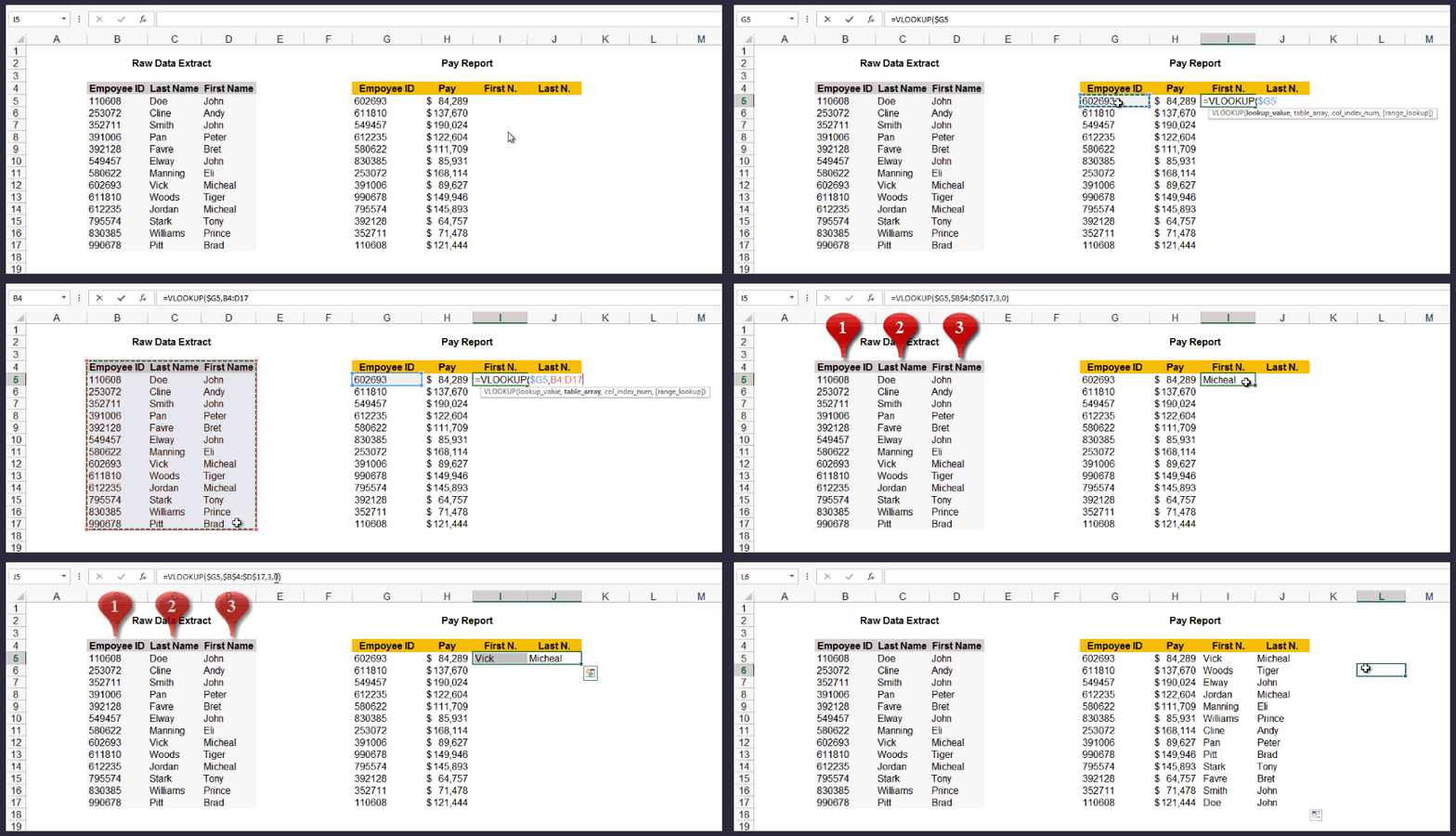
This function is used to locate specific information in a large dataset and retrieve that data from your Excel table. Click on the function option denoted by the ‘fx’ symbol in the tool, insert an equal to sign (=), and key in ‘VLOOKUP’. Once it’s typed in, a wizard box will pop-up automatically with a new set of box options. You can add your variables in the form of advances formulas like:
- Lookup_value
Type specific variables along with this function and they will be automatically shown as values in exact cells of the larger table of data points.
- Table Array
It highlights the range of the bigger table from where the information keyed in along with this function will be sourced. It marks the entire space of the data you want to pick.
- Col_index_num
This command box marks the column from where data needs to be picked-up.

Sum Function
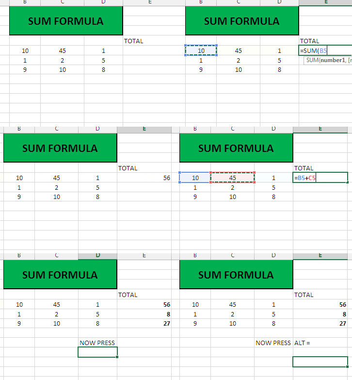
This function is most effectively used to sum a set of numbers in the specific column. The sum function has a dedicated button in the Home tab which can be used to add the selected items in a column.

Formula: =SUM(Select the range by placing the cursor on the desired box with the data and drag it till where the sum has to be calculated)
=DAYS
This function is a handy formula to detect the number of days between two dates. So, you can quickly check the exact number of days in a range, say, in a month easily.
Example: End Date (In A1 on Excel) October 12, 2019, Start Date (in A2 in Excel) March 10, 2019 = 216 days
Formula: =DAYS(End Date,Start Date)
AutoSum
This option is placed under the Home tab of MS Excel. For every day tasks, this function is handy for it contains hidden formula like Sum, Average, Count Numbers, Max, Min values, and more. Just navigate the Home tab in Excel, click on AutoSum and select any formula to calculate the desired information out of a selected range. This is denoted by ∑ icon in Excel.
IF Function
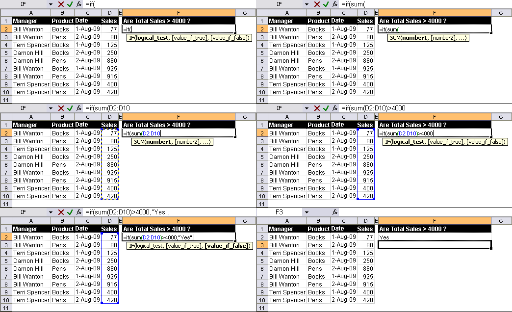
The IF function helps in extracting information of truth and false related to a parameter set in the variable box. The IF statement is formulated as:
- IF(Criteria,True,False value)
Once the criteria are added in the chosen column, then the answers are evaluated to determine the forecast to yield the best results accordingly.
- SUMIF Function
SUMIF function allows in seeing a certain set of data that match your criteria. The criteria are typed in a wizard box which contains the range tab, criteria tab, and the sum range tab. The range tab denotes the range you want to explore. The cell is identified by the criteria tab and the sum range tab adds up the data points matching your criteria.

COUNTIF Function
The only difference between the IF function and COUNTIF function is that this function does not add the matching values from the cells. It just retrieves and display the desired set to you.
COUNT
If you want to know which cells in a given range contain numeric values (numbers or dates), then all you need to do is use this handy function instead of wasting your time by counting them manually. The Excel COUNT function will show the result in a snap!
Formula: COUNT(value1, [value2], …
COUNTA
COUNTA checks the values of all cells in a given rage. What’s interesting is that this function, unlike the COUNT function, covers all cells regardless of their type. It not just only calculates numerical values but also counts dates, times, strings, logical values, errors, empty string, or text.
Formula: =COUNTA(value1, [value2], …)
TRIM
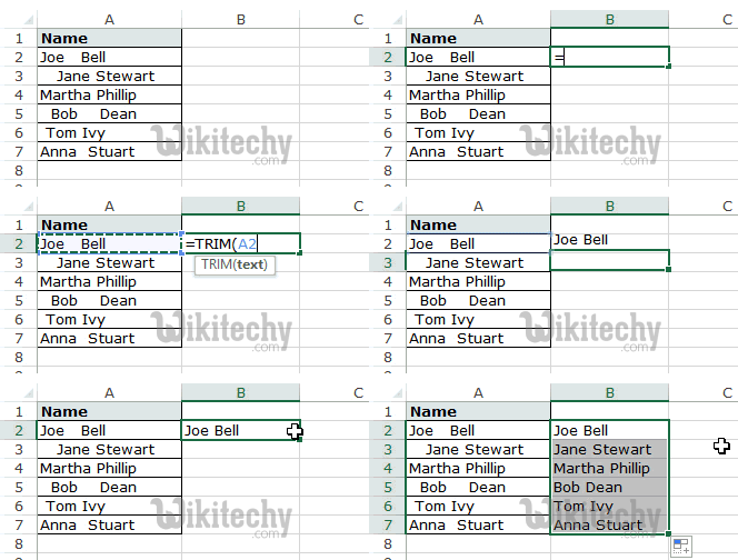
Sometimes, Excel formula calculations end-up showing some gaps. In case, you notice that the inserted Excel formulas are showing errors, then you should first check for extra spaces in the cells covered in your formula. At times, you may not realize but there can be multiple leading, trailing and in-between spaces that go unnoticed in your Excel sheet since the data set is huge.
In order to remove unwanted spaces in Excel quickly, the TRIM function is the easiest solution. Just put the formula and select the desired range (column/row) to eradicate any unwanted spaces.
Formula: =TRIM(text).

So, whether it’s calculating, doing spreadsheets, budgeting, making graphs, developing task lists and project management charts, or adding time logs with innovative pictures and even animations, Microsoft Excel is indeed a quintessential tool for all businesses today. From lists to charts to design mock-ups, the different applications of MS Excel are only seemingly beyond limits and always evolving with the software updates happening every now and then. Thanks to Apex Global’s training available for users to become an MS Excel pro, you can stay updated with the latest version of this versatile tool at all times. If you want to read more about the other features of MS Excel, click HERE.


